Complete Guide to R for DataDirect ODBC/JDBC

How can your business leverage the power of "R"? Justin Moore, a data scientist with 10 years of experience, explains the origins of "R" and gives a tutorial on how to implement it for ODBC/JDBC.
Introduction
What is R?
R is a statistical programming language, and runtime environment, used primarily for data analysis and graphics. R is distributed under the GNU project license. Within R, users will be able to make use of a wide range of statistical and graphical packages. R is available as free software under the terms of the Free Software Foundation’s GNU General Public License in source code form. It can be compiled on a large variety of UNIX, Linux, Windows, and Mac-OS systems.
What is RODBC/RJDBC?
RODBC and RJDBC are distributed (CRAN) R-packages that allow users to plug-in an applicable JDBC or ODBC driver to assist with database connectivity. Both packages can be obtained from the standard R-package repository (CRAN), and both packages are available for free. By combining RODBC/RJDBC with Progress DataDirect drivers, users can be sure that they now have access to a high-performing data access platform.
Prerequisites
Before you get started, make sure that the following software is installed and ready to use:
- R—Available here: https://www.r-project.org/
- Progress DataDirect Drivers (ODBC or JDBC) for your favorite data source—https://www.progress.com/datadirect-connectors
Run the installers for the software applications listed above, and then you will be ready to continue with R and DataDirect. (The examples below will be utilizing the DataDirect Spark driver.)
ODBC
The first step for ODBC is to set-up a new DSN. For more information on installing the driver or setting up a DSN please consult the DataDirect documentation for your driver. Once the DSN has been created, make a note of the DSN name, you will need it later. For this example, my DSN is called “Spark Next”
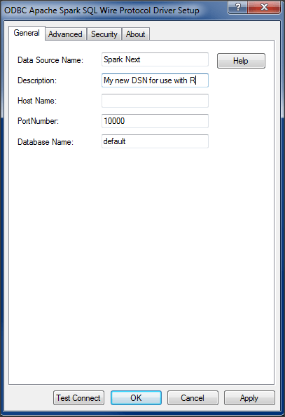
After your DSN has been configured, use the “Test Connect” button to ensure that you can successfully connect to your data source. Next, go ahead and launch R.
Note: Instructions below are applicable to the RGui application
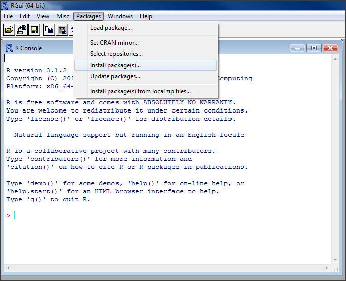
Before continuing, we will need to install the RODBC package. To do so:
- Click “Packages” à Install package(s)… from the RGui Toolbar

- If you have not already selected a mirror for CRAN downloads, do so by selecting a mirror that will best serve your geographic location
- Select “RODBC” from the package list
- The RODBC package has been successfully installed
- If you do not wish to use the CRAN distribution installation through RGui, RODBC can also be found here: https://cran.r-project.org/web/packages/RODBC/index.html
Making a Connection
The next phase will involve using our DSN that we created early to establish a connection (via an R script) to our database.
Start by creating a new R script.
Making a connection is easy. The sample R code below will give you a good idea of how it works. Don’t forget to include the “library(RODBC)” call to include the necessary packages and to replace “Spark Next” with your DSN name”
library(RODBC)
# Make a connection using your DSN name
conn <- odbcConnect("Spark Next")
After you have established a connection, it is probably a good idea to go ahead and include the disconnect call (just so you don’t forget). This can be done with the following script code:
close(conn)
Now that we have a connection, we can insert more code in between our open and close call to manipulate our data. Take a look at the sample R-script below.
library(RODBC)
# Make a connection using your DSN name
conn <- odbcConnect("Spark Next")
# Execute a SQL Tables call
sqlTables(conn)
# Execute a SQL columns call on the table with our energy data
sqlColumns(conn, "energyconsumption")
# Bind the results of a SQL query for plotting
data <- sqlQuery(conn, "SELECT * FROM energyconsumption WHERE country IN ('China', 'United States', 'Canada', 'France', 'Germany', 'Italy', 'Japan')")
# Attach the data for plotting access
attach(data)
# Partition our plot screen for multiple plots
par(mfrow=c(2,2))
# Plot overall data usage from 2 years, with a box-plot for 2008
plot(data$country, data$'1980', main="Total Energy Consumption in 1980", xlab="Country", ylab="Usage (Quadrillion BTU)", pch=19)
plot(data$country, data$'2008', main="Total Energy Consumption in 2008", xlab="Country", ylab="Usage (Quadrillion BTU)", pch=19)
boxplot(data$'2008', main="Total Energy Distribution (2008)", ylab="Usage (Quadrillion BTU)")
# Create a new plot window
dev.new()
# Plot overall energy consumption for 2008 via a histogram (show density lines)
hist(data$'2008', prob=TRUE, main="Energy Distribution Density - 2008", xlab="Usage (Quadrillion BTU)")
lines(density(data$'2008'))
lines(density(data$'2008', adjust=2), lty="dotted")
# Close the connection to our database
close(conn)
The comments above (marked with #) will give you a good idea of the general workflow:
- Make a connection
- Issue a query using sqlQuery and store the results
- Attach the data, and generate a plot
JDBC
JDBC Connections are also easy to make when utilizing the RJDBC package. To get started:
- Click “Packages” à Install package(s)… from the RGui Toolbar
- If you have not already selected a mirror for CRAN downloads, do so by selecting a mirror that will best serve your geographic location
- Select “RJDBC” from the package list
- The RJDBC package has been successfully installed
- If you do not wish to use the CRAN distribution installation through RGui, RJDBC can also be found here: https://cran.r-project.org/web/packages/RJDBC/index.html
Once RJDBC has been installed, you simply need to make a note of where your JDBC driver is located on your local file system. Once you have the path, make a note of it for your RJDBC R Script.
Create a new R-script.
Making a Connection
Making a connection is easy. The sample R code below will give you a good idea of how it works. Don’t forget to include the “library(RJDBC)” call to include the necessary packages.
RJDBC connections require two steps. First, you have to tell the package where your JDBC driver (.jar file) is located. Do so by passing in the path to the .jar file (keeping in mind to properly escape \ characters or replace them with / .
Once that is done, go ahead and create a connection object by calling dbConnect. For more information on forming your JDBC connection URL, consult your DataDirect driver documentation.
library(RJDBC)
# Tell R where your JDBC driver is located
driver <- JDBC("com.ddtek.jdbc.sparksql.SparkSQLDriver", "C:/Users/jmoore/Desktop/R POC/Spark Drivers/JDBC/sparksql.jar", identifier.quote="`")
# Make a connection using your JDBC driver and connection URL
conn <- dbConnect(driver, "jdbc:datadirect:sparksql://hostname:11111;Database=databaseName;", "username", "password")
After you have established a connection, the general workflow will be similar to the ODBC instructions above:
- Execute any catalog calls (e.g. dbListTables()
- Execute a query using dbGetQuery and store the results
- Attach the results
- Generate plots or perform analysis
The sample R-script below will be enough to get you started:
library(RJDBC)
# Tell R where your JDBC driver is located
driver <- JDBC("com.ddtek.jdbc.sparksql.SparkSQLDriver", "C:/Users/jmoore/Desktop/R POC/Spark Drivers/JDBC/sparksql.jar", identifier.quote="`")
# Make a connection using your JDBC driver and connection URL
conn <- dbConnect(driver, "jdbc:datadirect:sparksql://<hostname>:<portnumber>;Database=perf;", "username", "password")
# Execute a SQL Tables call
dbListTables(conn)
# Bind the results of a SQL query for plotting
data <- dbGetQuery(conn, "SELECT * FROM energyconsumption WHERE country IN ('China', 'United States', 'Canada', 'France', 'Germany', 'Italy', 'Japan')")
# Attach the data for plotting access
attach(data)
# Create a new plot window
dev.new()
# Plot overall energy consumption for 2008 via a histogram (show density lines)
hist(data$'2008', prob=TRUE, main="Energy Distribution Density - 2008", xlab="Usage (Quadrillion BTU)")
lines(density(data$'2008'))
lines(density(data$'2008', adjust=2), lty="dotted")
# Close the connection to our database
dbDisconnect(conn)
Additional Considerations
For additional documentation on the RODBC and RJDBC API’s see the links below:
RODBC: https://cran.r-project.org/web/packages/RODBC/RODBC.pdf
RJDBC: https://cran.r-project.org/web/packages/RJDBC/RJDBC.pdf
Now You’re Finished!
With your R package, you can leverage your data analytics and graphics in new and exciting ways. The next step is to integrate with your favorite data source through an ODBC/JDBC connector. Luckily, you’re in the right place because our drivers are the fastest in the industry. Speed is the key in any business and we stand by our standard with award winning technical support. Skeptical? Pick up a free trial today and find out yourself.

